import numpy as np

%matplotlib inline
import matplotlib.pyplot as plt
from jupyterthemes import jtplot

jtplot.style(context="talk", fscale=1.4, spines=False, gridlines="--")

from pychangcooper import SynchrotronCooling_ContinuousPLInjection

Synchrotron cooling

In the case of simple synchrotron cooling, the diffusion/dispersion term is zero. However, we will have a source term, \(Q(\gamma, t)\). Thus we have the simple case of:

\[\frac{\partial N\left(\gamma, t\right)}{\partial t} = \frac{\partial }{\partial \gamma} B \left(\gamma, t \right)N\left(\gamma, t\right) + Q(\gamma, t)\]

The synchrotron cooling class computes the cooling time of the electrons and sets the time step of the solver to the cooling time of the highest energy electron which evolves the most.

Solution

Setup the solver

First we set the solver with the initial physical parameters.

synch_cool = SynchrotronCooling_ContinuousPLInjection(
    B=1e10,
    index=-3.5,
    gamma_injection=1e3,
    gamma_cool=500,
    gamma_max=1e5,
    store_progress=True,
)

Solving

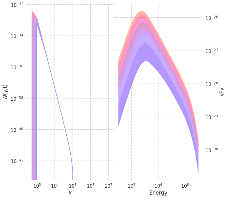
The solver automatically sets of the number of iterations such that the dynamical time equals the cooling time. If an array of photon energies are also passed, then the photon spectrum that is emitted by the electrons is also computed.

synch_cool.run(photon_energies=np.logspace(1, 7, 50))

synch_cool.plot_photons_and_electrons(skip=20, alpha=0.7, cmap="vaporwave")