[1]:
import numpy as np

%matplotlib inline
import matplotlib.pyplot as plt
from jupyterthemes import jtplot

jtplot.style(context="talk", fscale=1.4, spines=False, gridlines="--")

from pychangcooper import CoolingAcceleration
Generic Cooling and Acceleration
For a generic heating/cooling and acceleration problem, we rewrite the Fokker-Planck equation as:
where:
Here we specify \(C \left( \gamma \right) = C_{0} \gamma^{a}\) and \(D\left( \gamma \right) = \frac{1}{2 t_{\text{acc}}} \gamma^{b}\) where the acceleration time is \(t_{\text{acc}}\). The steady-state solution for this problem (given no injection or escape) is
.
If we let \(a=b=2\), an electron of energy \(\gamma\) will cool in a characteristic time \(t_{\text{cool}}(\gamma) = 1 / \left(C_0 \gamma \right)\), thus when the cooling time is equal to the acceleration time, and electron will have an equilibrium energy \(\gamma_{\text{e}} = \frac{1}{t_{\text{acc}}C_0}\).
Solving the equation
Setting an initial distribution
We will start with an initial flat electron distribution at low energy and let it evolve for \(50\cdot t_{\text{acc}}\).
[2]:
n_grid_points = 300

init_distribution = np.zeros(n_grid_points)


for i in range(30):

    init_distribution[i + 1] = 1.0
Create the solver
We set \(C_0 = 1\) and \(t_{\text{acc}} = 10^{-4}\) and thus \(\gamma_{\text{e}} = 10^4\).
[3]:
generic_ca = CoolingAcceleration(
    n_grid_points=n_grid_points,
    C0=1.0,
    t_acc=1e-4,
    cooling_index=2.0,
    acceleration_index=2.0,
    initial_distribution=init_distribution,
    store_progress=True,
)
Run the solver:
[4]:
for i in range(45):

    generic_ca.solve_time_step()
Plot the history of the solution
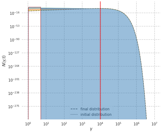
[5]:
fig = generic_ca.plot_evolution(
    skip=5, alpha=0.5, cmap="Set1", show_initial=True, show_final=True, show_legend=True
)

ax = fig.get_axes()[0]

# plot the equilbrium solution
ax.axvline(1e4, color="red", lw=4, zorder=100, alpha=0.5)
[5]:
<matplotlib.lines.Line2D at 0x7f768b52d750>
[ ]: